EXA2PRO: HiePACS parallel linear solvers
Table of Contents
- 1. Introduction to GNU Guix
- 2. Chameleon dense linear solver
- 3. PaStiX sparse direct solver
- 4. MaPHyS sparse hybrid solver
- 4.1. Installation
- 4.2. Using MaPHyS drivers to test hybrid solvers behaviors
- 4.2.1. A first execution
- 4.2.2. An actual hybrid method
- 4.2.3. Exploit SPD properties
- 4.2.4. Try running on more subdomains
- 4.2.5. Use a robust algebraic domain decompostion
- 4.2.6. Backward and forward error analysis
- 4.2.7. Sparse direct solver
- 4.2.8. Display more info
- 4.2.9. Sparsification
- 4.2.10. Force GMRES
- 4.2.11. Multiple right-hand sides (
fabulous) - 4.2.12. Larger testcase
- 4.2.13. MPI + Threads
- 4.2.14. Coarse Grain Correction
- 4.3. Using MaPHyS in your C/Fortran code (soon C++)
- 4.4. Issues
This is a hands-on tutorial for introducing some of the Inria HiePACS team parallel linear solvers.
We will install the softwares thanks to GNU Guix for the sake of reproducibility.
We will show how to use them on a supercomputer, here PlaFRIM. Notice that on this cluster Guix has been installed by administers.
Lets login on PlaFRIM
ssh plafrim
1. Introduction to GNU Guix
1.1. Key features
- reproducibility: same code on laptop & cluster
- versatility: “package management”, container provisioning, etc.
- transactional upgrades and rollback
- PlaFRIM support!
How to install Guix:
# Guix requires a running GNU/Linux system, GNU tar and Xz.
gpg --keyserver pgp.mit.edu --recv-keys 3CE464558A84FDC69DB40CFB090B11993D9AEBB5
wget https://git.savannah.gnu.org/cgit/guix.git/plain/etc/guix-install.sh
chmod +x guix-install.sh
sudo ./guix-install.sh
1.2. Installation, Removal
# look for available packages
guix search ^openmpi

# list installed packages
guix package -I

# install packages
guix install hwloc gcc-toolchain
which lstopo

# where are located installed files
ls ~/.guix-profile/bin
cat ~/.guix-profile/etc/profile

# remove packages
guix remove hwloc gcc-toolchain

# list iterations
guix package --list-generations

# come back to a previous state of packages installation
guix package --roll-back
guix package --switch-generation=+1
1.3. Update and Upgrade
# update Guix and the list of available packages
guix pull

# upgrade installed packages
guix upgrade
1.4. Reproduce
# current guix commit
guix --version

# rewind packages recipies to a past version
guix pull --commit=adfbba4

# save current guix state (commits of guix and of additional channels)
guix describe -f channels > channels-date.scm

# restore guix state (+ external channels) to a past version
guix pull --allow-downgrades -C channels-date.scm
1.5. Environment
# setup a development environment ready to be used for compiling petsc (i.e. compilers + dependencies)
guix environment petsc

# use the following to get an environment isolated from the the system one
guix environment --pure petsc -- /bin/bash --norc
1.6. Docker and Singularity
# create docker image
guix pack -f docker petsc -S /bin=bin --entry-point=/bin/bash

# create singularity image
guix pack -f squashfs petsc -S /bin=bin --entry-point=/bin/bash
1.7. Get additional Inria packages
See our Gitlab project guix-hpc-non-free where packages for installing Chameleon, PaStiX and MaPHyS can be found.
It is necessary to add a channel to get new packages. Create a ~/.config/guix/channels.scm file with the following snippet:
(cons (channel
    (name 'guix-hpc-non-free)
    (url "https://gitlab.inria.fr/guix-hpc/guix-hpc-non-free.git"))
  %default-channels)
Update guix packages definition
guix pull
Update new guix in the path
PATH="$HOME/.config/guix/current/bin${PATH:+:}$PATH"
hash guix
For further shell sessions, add this to the ~/.bash_profile file
export PATH="$HOME/.config/guix/current/bin${PATH:+:}$PATH"
export GUIX_LOCPATH="$HOME/.guix-profile/lib/locale"
New packages are now available
guix search ^starpu
guix search ^chameleon
guix search ^pastix
guix search ^maphys
2. Chameleon dense linear solver
2.1. Installation
2.1.1. Using Guix
guix install openssh openmpi chameleon --with-input=openblas=mkl
2.1.2. Using CMake
Without Guix one has to get installed the following components:
- CMake
- GNU GCC
- MPI (e.g. Open MPI),
- Intel MKL (or OpenBLAS),
- Nvidia CUDA/cuBLAS (optional),
- StarPU (e.g. latest release 1.3.7)
Most of them should be already provided through modules and for StarPU:
# on your laptop
wget https://files.inria.fr/starpu/starpu-1.3.7/starpu-1.3.7.tar.gz
scp starpu-1.3.7.tar.gz plafrim:

# install starpu on the cluster
ssh plafrim

# load the modules for compilers (C/C++, Fortran), MPI, CUDA
module purge
module add build/cmake/3.15.3
module add compiler/gcc/9.3.0
module add compiler/cuda/11.2
module add hardware/hwloc/2.1.0
module add mpi/openmpi/4.0.2
module add linalg/mkl/2019_update4

tar xvf starpu-1.3.7.tar.gz
cd starpu-1.3.7
export STARPU_ROOT=$PWD/install
./configure --prefix=$STARPU_ROOT
make -j5 install
Then one can install Chameleon using CMake, e.g.
# on your laptop
wget https://gitlab.inria.fr/solverstack/chameleon/uploads/6115a9dd4dc21da4aed13a14b2de49d3/chameleon-1.0.0.tar.gz
scp chameleon-1.0.0.tar.gz plafrim:

# install chameleon on the cluster
ssh plafrim
tar xvf chameleon-1.0.0.tar.gz
cd chameleon-1.0.0
mkdir build && cd build

module purge
module add build/cmake/3.15.3
module add compiler/gcc/9.3.0
module add compiler/cuda/11.2
module add hardware/hwloc/2.1.0
module add mpi/openmpi/4.0.2
module add linalg/mkl/2019_update4
# starpu should be available in the environement, for example with
export PKG_CONFIG_PATH=$STARPU_ROOT/lib/pkgconfig:$PKG_CONFIG_PATH

# configure, make, install
cmake .. -DCHAMELEON_USE_MPI=ON -DCHAMELEON_USE_CUDA=ON -DBLA_VENDOR=Intel10_64lp_seq -DCMAKE_INSTALL_PREFIX=$PWD/install
make -j5 install

# test
mpiexec -np 2 ./testing/chameleon_stesting -o gemm -n 2000 -t 2
2.2. Using Chameleon to test dense linear algebra performances
Chameleon provides executables to test dense linear algebra algorithms. These drivers allow to
- check numerical results,
- time the execution and
- deduce the performance by computing the gigaflop rate, i.e. the number of operations performed by seconds.
By default four executables are provided, one for each arithmetic
precision, chameleon_stesting for simple precision, and the
equivalent for other precisions with d (double), c (complex simple), z
(complex double).
To get all parameters
chameleon_stesting --help
See also in the documentation the available algorithms which can be checked.
For example to check the performances of GEMM in simple or double precision using 2 threads (using the guix installation here)
mpiexec -np 1 chameleon_stesting -o gemm -n 3200 -t 2
mpiexec -np 1 chameleon_dtesting -o gemm -n 3200 -t 2
is performed around 0.25 s for simple and 0.5 s for double and gives around 270 Gflop/s and 130 Gflop/s respectively.
To check a Cholesky
mpiexec -np 1 chameleon_stesting -o potrf -n 3200 -t 2
which give around 245 Gflop/s in this configuration.
Lets reserve some machines with Slurm to check performances on entire nodes
# slurm reservation
salloc --nodes=2 --time=01:00:00 --constraint bora --exclusive --ntasks-per-node=1 --threads-per-core=1

# check nodes obtained
mpiexec hostname
Chameleon on one node
mpiexec -np 1 chameleon_stesting -o potrf -n 3200,6400,16000,32000
gives
Id;Function;threads;gpus;P;Q;nb;uplo;n;lda;seedA;time;gflops
0;spotrf;35;0;1;1;320;121;3200;3200;846930886;1.301987e-02;8.393163e+02
1;spotrf;35;0;1;1;320;121;6400;6400;1681692777;3.153522e-02;2.771562e+03
2;spotrf;35;0;1;1;320;121;16000;16000;1714636915;3.651932e-01;3.739011e+03
3;spotrf;35;0;1;1;320;121;32000;32000;1957747793;3.038234e+00;3.595240e+03
Chameleon on two nodes
mpiexec -np 2 chameleon_stesting -o potrf -n 3200,6400,16000,32000,64000
gives
Id;Function;threads;gpus;P;Q;nb;uplo;n;lda;seedA;time;gflops
0;spotrf;35;0;1;2;320;121;3200;3200;846930886;1.988709e-02;5.494916e+02
1;spotrf;35;0;1;2;320;121;6400;6400;1681692777;4.519280e-02;1.933976e+03
2;spotrf;35;0;1;2;320;121;16000;16000;1714636915;2.688228e-01;5.079411e+03
3;spotrf;35;0;1;2;320;121;32000;32000;1957747793;2.119557e+00;5.153520e+03
4;spotrf;35;0;1;2;320;121;64000;64000;424238335;1.366869e+01;6.392958e+03
Try with different algorithms to compare
mpiexec -np 1 chameleon_stesting --nowarmup -o gemm -n 3200,6400,16000,32000
mpiexec -np 2 chameleon_stesting --nowarmup -o gemm -n 32000

mpiexec -np 1 chameleon_stesting --nowarmup -o symm -n 3200,6400,16000,32000
mpiexec -np 2 chameleon_stesting --nowarmup -o symm -n 32000

mpiexec -np 1 chameleon_stesting --nowarmup -o getrf -n 3200,6400,16000,32000
mpiexec -np 2 chameleon_stesting --nowarmup -o getrf -n 32000

mpiexec -np 1 chameleon_stesting --nowarmup -o geqrf -n 3200,6400,16000,32000
mpiexec -np 2 chameleon_stesting --nowarmup -o geqrf -n 32000

mpiexec -np 1 chameleon_stesting --nowarmup -o gels -n 3200,6400,16000,32000
mpiexec -np 2 chameleon_stesting --nowarmup -o gels -n 32000
Be aware that Chameleon follows a 2D block-cyclic distribution of the data over MPI processes which parameters can be handled by the user with the -P option. Depending on the matrices size, form and number of MPI processes, this parameter can play a key role over performances.
These testing drivers do not allow to check eigenvalue problems,
i.e. gesvd and heevd, for now because they are not ready to be used
in a MPI distributed context. Nevertheless usage of the gesvd and
heevd algorithms in a shared memory context is fine. Getting good
performances on several nodes on these eigenvalue problems is a
future work in Chameleon.
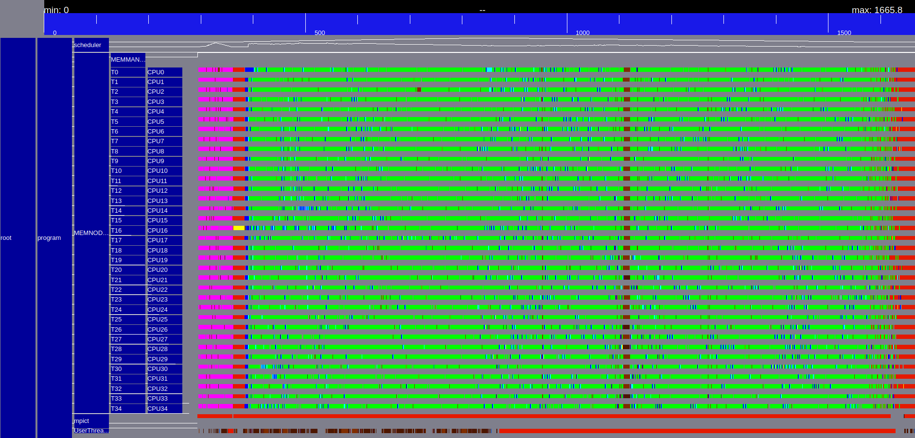
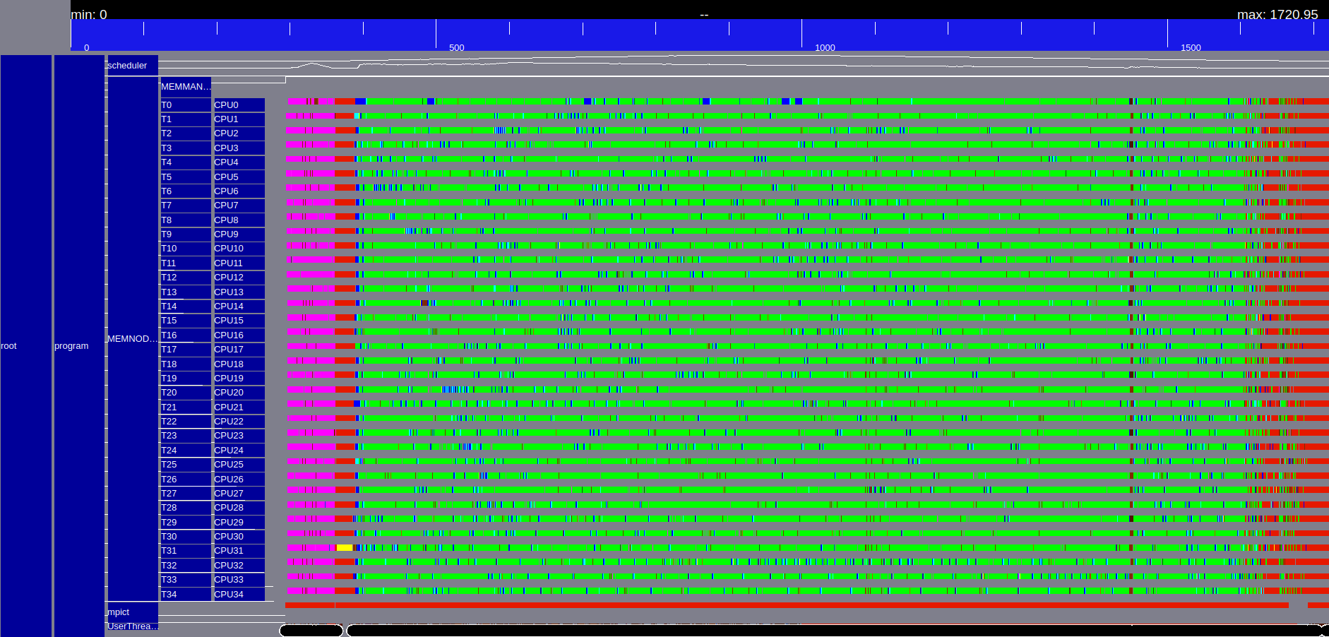
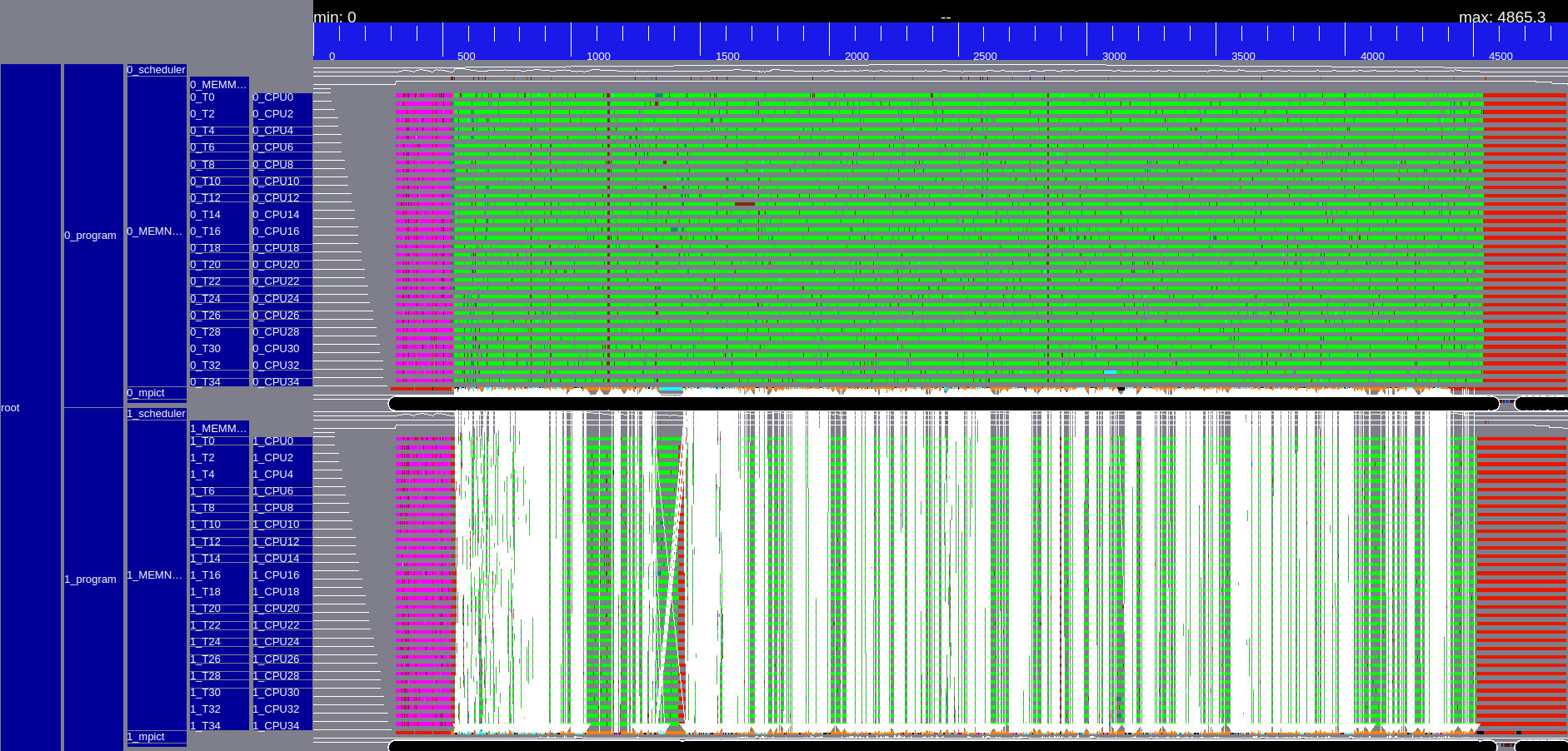
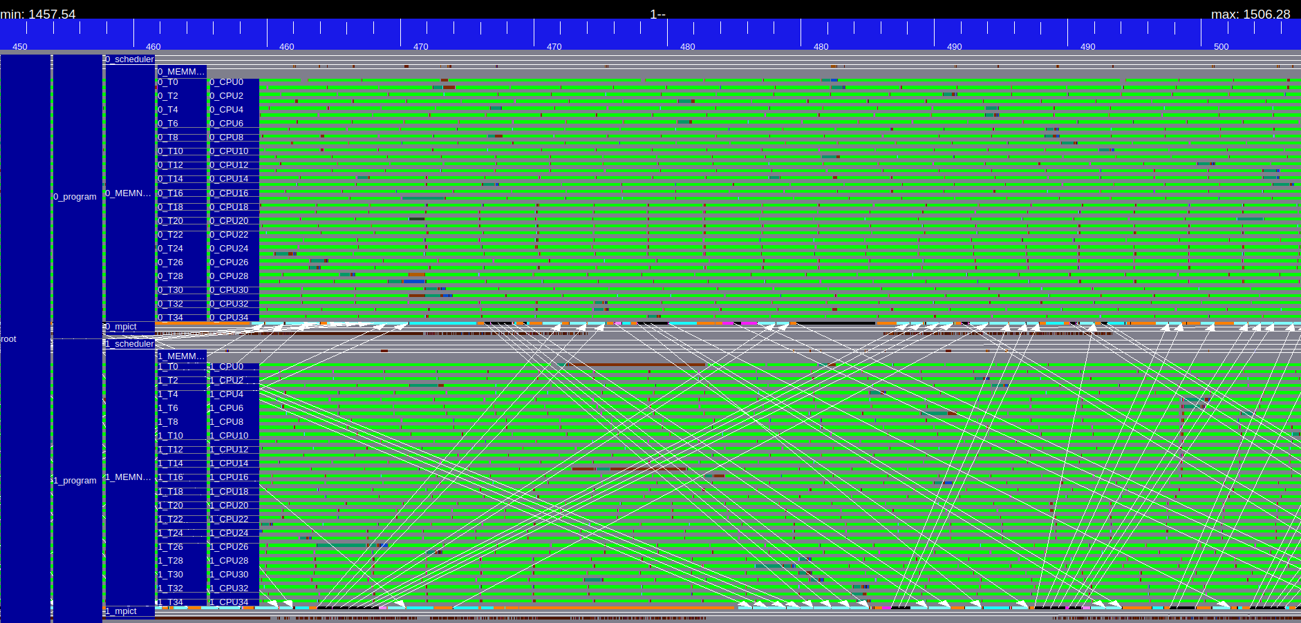
2.3. Analyzing performances with execution traces
Lets observe now some execution traces thanks to StarPU and ViTE.
By default Chameleon is built without traces enabled (because it slows done a little bit the execution). To enable this feature one has to install StarPU with FxT component, see the documentation.
We choose to install it with Guix here
# remove the default version of chameleon
guix remove chameleon

# install a version with traces enabled
guix install chameleon --with-input=openblas=mkl --with-input=starpu=starpu-fxt starpu-fxt
# slurm reservation
salloc --nodes=2 --time=01:00:00 --constraint bora --exclusive --ntasks-per-node=1 --threads-per-core=1

# indicate where to generate profiling files
export STARPU_FXT_PREFIX=$PWD/

# Chameleon potrf execution
mpiexec -np 1 chameleon_stesting --nowarmup -o potrf -n 24000 -b 480 --trace

# generate the paje trace
starpu_fxt_tool -i prof_file_pruvost_* -o chameleon_spotrf.paje

# Chameleon posv execution
mpiexec -np 1 chameleon_stesting --nowarmup -o posv -n 24000 -b 480 --trace
starpu_fxt_tool -i prof_file_pruvost_* -o chameleon_sposv.paje

# Chameleon gemm execution
mpiexec -np 2 chameleon_stesting --nowarmup -o gemm -n 24000 -b 480 --trace
starpu_fxt_tool -i prof_file_pruvost_* -o chameleon_sgemm.paje
One can now vizualize the trace with ViTE
# on your laptop
sudo apt install vite

# get the paje file back to your laptop
scp plafrim:*.paje .

# load the file with ViTE
vite chameleon_spotrf.paje &
vite chameleon_sposv.paje &
vite chameleon_sgemm.paje &
| POTRF | POSV |
 |
 |
| GEMM | GEMM zoom |
 |
 |
2.4. Using Chameleon with GPUs
First install Chameleon with CUDA enabled, for example with Guix
guix remove chameleon starpu-fxt

guix install chameleon-cuda --with-input=openblas=mkl --with-input=starpu-cuda=starpu-cuda-fxt starpu-cuda-fxt
# slurm reservation
salloc --nodes=1 --time=01:00:00 --constraint sirocco --exclusive --ntasks-per-node=1 --threads-per-core=1

# indicate where to generate profiling files
export STARPU_FXT_PREFIX=$PWD/

# use ld preload for Guix to get path to nvidia drivers on the node with GPUs
export LD_PRELOAD="/usr/lib64/libcuda.so /usr/lib64/libnvidia-fatbinaryloader.so.440.33.01"

# Chameleon potrf execution
mpiexec -np 1 chameleon_stesting --nowarmup -o potrf -n 76800 -b 1920 -g 2 --trace
delivers something like 22 Tflop/s on 2 V100.
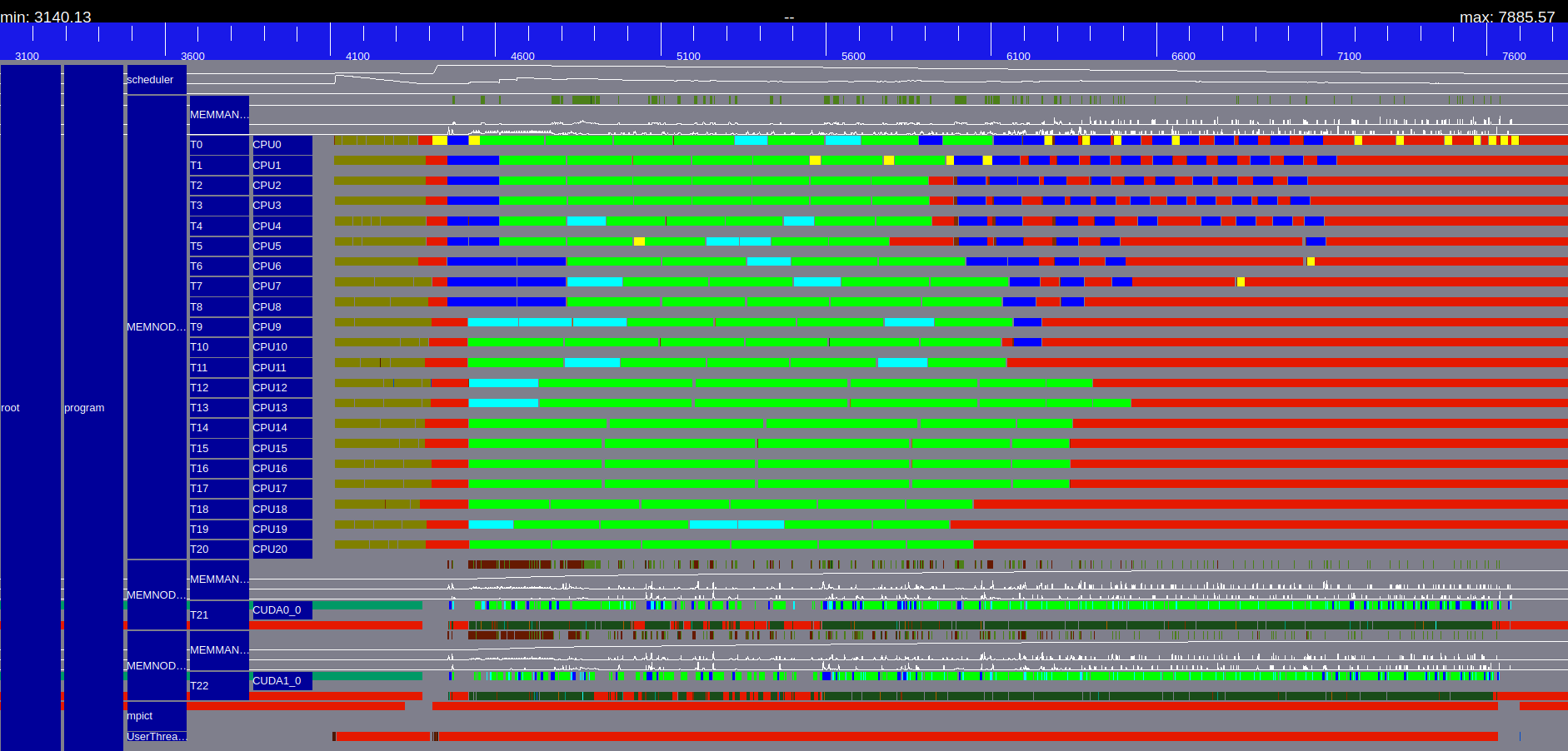
Figure 1: Execution trace of Chameleon spotrf N=32000, B=1600
2.5. Using Chameleon in your C/C++ project
2.6. Issues
Do not hesitate to submit issues by sending an email.
3. PaStiX sparse direct solver
The solver is currently evolving, and two versions are availables. The first historical version is available on the Inria forge. This version will become deprecated to the benefit of the current version under development, and publicly available on Gitlab. The main difference is the MPI support that is not yet fully integrated to the new PaStiX, but it includes all recent development on low-rank compression and runtime support for GPUs.
3.1. Installation
3.1.1. Using Guix
guix install openssh openmpi pastix --with-input=openblas=mkl
3.1.2. Using CMake
PaStiX needs several libraries to be compiled and installed on your cluster:
- An implementation of the Message Passing Interface 2.0 standard like MPICH, Open MPI, …
- An implementation of the Basic Linear Algebra Subroutines standard (BLAS) like OpenBLAS, ACML, INtel MKL, …
- A library to compute ordering in order to reduce fill-in and increase parallelism like Scotch, PT-Scotch or Metis. The user can also provide it's own ordering.
- The Hardware Locality library (HwLoc) is not required but highly recommended especially if PaStiX is compiled with threads support. It will give an uniform view of the architecture to the solver (Hide hyper-threading, linearize core numbering, …).
- A runtime system PaRSEC or StarPU (optional). Installation example of StarPU has been done in the previous section about Chameleon.
# on your laptop
wget https://gitlab.inria.fr/solverstack/pastix//uploads/98ce9b47514d0ee2b73089fe7bcb3391/pastix-6.1.0.tar.gz
scp pastix-6.1.0.tar.gz plafrim:

ssh plafrim

# load the modules for dependencies
module purge
module add build/cmake/3.15.3
module add compiler/gcc/8.2.0
module add compiler/cuda/10.2
module add hardware/hwloc/2.1.0
module add mpi/openmpi/4.0.2
module add linalg/mkl/2019_update4
module add partitioning/scotch/int64/6.0.9
module add trace/eztrace/1.1-9
module add runtime/parsec/master/shm-cuda
module add trace/fxt/0.3.11
module add runtime/starpu/1.3.7/mpi-cuda-fxt

tar xvf pastix-6.1.0.tar.gz
cd pastix-6.1.0
# patch to apply to cmake_modules/morse_cmake/modules/find/FindPARSEC.cmake +567
#  list(APPEND REQUIRED_LIBS "${CUDA_CUBLAS_LIBRARIES};${CUDA_LIBRARIES}")
mkdir build && cd build

# configure, make, install
export PASTIX_ROOT=$PWD/install
cmake .. -DPASTIX_ORDERING_SCOTCH=ON -DPASTIX_WITH_PARSEC=ON -DPASTIX_WITH_STARPU=ON -DPASTIX_WITH_CUDA=ON -DPASTIX_WITH_MPI=ON -DPASTIX_WITH_EZTRACE=ON -DBLA_VENDOR=Intel10_64lp_seq -DBUILD_SHARED_LIBS=ON -DCMAKE_INSTALL_PREFIX=$PASTIX_ROOT
make -j5 install

# test
./example/simple --lap 1000 --threads 2
3.2. Using PaStiX to test sparse linear algebra performances
# slurm reservation
salloc --nodes=1 --time=01:00:00 --constraint sirocco --exclusive --ntasks-per-node=1 --threads-per-core=1

# check nodes obtained
mpiexec hostname
To run a simple example on a 2D Laplacian of size 1000
# test laplacian
mpiexec --map-by ppr:1:node:pe=40 $PASTIX_ROOT/examples/simple --lap 100000
3.2.1. Cholesky factorization
Perform Cholesky factorization on matrices, see parameters:
-f 0to apply a Cholesky facorization-sto choose the runtime as scheduler (1 for native pastix, 2 parsec, 3 starpu)-gnumber of gpus-iminimum block size to avoid too small blocks on the gpus
# static scheduling without gpus (700 GFlops/s)
mpiexec --map-by ppr:1:node:pe=40 $PASTIX_ROOT/examples/bench_facto --threads 40 -f 0 --mm /projets/matrix/GHS_psdef/audikw_1/audikw_1.mtx

# using parsec runtime with 1 or 2 gpus (900 GFlops/s and 1.1 TFlops/s)
mpiexec --map-by ppr:1:node:pe=40 $PASTIX_ROOT/examples/bench_facto --threads 40 -f 0 --mm /projets/matrix/GHS_psdef/audikw_1/audikw_1.mtx -s 2 -g 1 -i iparm_min_blocksize 920 -i iparm_max_blocksize 920
mpiexec --map-by ppr:1:node:pe=40 $PASTIX_ROOT/examples/bench_facto --threads 40 -f 0 --mm /projets/matrix/GHS_psdef/audikw_1/audikw_1.mtx -s 2 -g 2 -i iparm_min_blocksize 920 -i iparm_max_blocksize 920
See also these hints to optimize pastix with GPUs.
3.2.2. LU factorization
Perform LU factorization on matrices, see parameters:
-f 2to apply a LU facorization-sto choose the runtime as scheduler (1 for native pastix, 2 parsec, 3 starpu)-gnumber of gpus-iminimum block size to avoid too small blocks on the gpus-dthe compression low-rank precision criterion
# static scheduling without gpus (440 GFlops/s)
mpiexec --map-by ppr:1:node:pe=40 $PASTIX_ROOT/examples/bench_facto --threads 40 -f 2 --mm /projets/matrix/Bourchtein/atmosmodj/atmosmodj.mtx

# using parsec runtime with 2 gpus (1 TFlops/s)
mpiexec --map-by ppr:1:node:pe=40 $PASTIX_ROOT/examples/bench_facto --threads 40 -f 2 --mm /projets/matrix/Bourchtein/atmosmodj/atmosmodj.mtx -s 2 -g 2 -i iparm_min_blocksize 920 -i iparm_max_blocksize 920

# using compression low-rank (1 TFlops/s, considering full-rank kernels number of operations)
mpiexec --map-by ppr:1:node:pe=40 $PASTIX_ROOT/examples/bench_facto --threads 40 -f 2 --mm /projets/matrix/Bourchtein/atmosmodj/atmosmodj.mtx -i iparm_compress_when 2 -d dparm_compress_tolerance 1e-8
3.2.3. Generate traces with EZTrace
When StarPU is used we can generate FxT traces the same way we have seen in the chameleon section.
There is an alternative method, more generic, that works with any runtime, using EZtrace.
First EZtrace should be installed and -DPASTIX_WITH_EZTRACE=ON
must be used during the project configuration.
Before execution we tell eztrace which kernels family we want to time, here pastix tasks:
# setup eztrace modules for traces
export EZTRACE_TRACE="kernels"
export EZTRACE_LIBRARY_PATH=$PWD/kernels
Perform the execution
mpiexec --map-by ppr:1:node:pe=40 $PASTIX_ROOT/examples/bench_facto --threads 40 -f 0 --mm /projets/matrix/GHS_psdef/audikw_1/audikw_1.mtx
Generate the trace, see kernels statistics
eztrace_stats -o output pruvost_eztrace_log_rank_1
eztrace_convert -o output pruvost_eztrace_log_rank_1
mv output.trace audikw_1.paje
This paje trace can be read with ViTE.
3.3. Using PaStiX in your C/C++ project
3.4. Issues
Do not hesitate to submit issues by sending an email.
4. MaPHyS sparse hybrid solver
4.1. Installation
4.1.1. Using Guix
guix install openssh openmpi maphys --with-input=mumps-openmpi=mumps-mkl-openmpi --with-input=openblas=mkl --with-input=lapack=mkl
export MAPHYS_ROOT=`guix package -I maphys |gawk '{print $4}'`
4.1.2. Using CMake
MaPHyS needs several libraries to be compiled and installed on your cluster:
- An implementation of the Message Passing Interface 2.0 standard like MPICH, Open MPI, …
- An implementation of the Basic Linear Algebra Subroutines standard (BLAS, LAPACK and ScaLAPACK) like OpenBLAS, ACML, Intel MKL, …
- Scotch library to compute ordering in order to reduce fill-in and increase parallelism. The user can also provide it's own ordering.
- The Hardware Locality library (HwLoc).
- A sparse direct solver MUMPS or PaStiX (6.0.3 for now, compatibility issue).
# on your laptop
wget https://gitlab.inria.fr/solverstack/pastix//uploads/bd29252eb0390fa7bcb4e4d238c5b30a/pastix-6.0.3.tar.gz
wget http://morse.gforge.inria.fr/maphys/maphys-1.0.0.tar.gz
scp pastix-6.0.3.tar.gz plafrim:
scp maphys-1.0.0.tar.gz plafrim:

ssh plafrim

# load the modules for dependencies
module purge
module add build/cmake/3.15.3
module add compiler/gcc/8.2.0
module add hardware/hwloc/2.1.0
module add mpi/openmpi/4.0.2
module add linalg/mkl/2019_update4
module add partitioning/scotch/int64/6.0.9


# install pastix
tar xvf pastix-6.0.3.tar.gz
cd pastix-6.0.3
# patch to apply to cmake_modules/morse_cmake/modules/find/FindPARSEC.cmake +567
#  list(APPEND REQUIRED_LIBS "${CUDA_CUBLAS_LIBRARIES};${CUDA_LIBRARIES}")
mkdir build && cd build
export PASTIX_ROOT=$PWD/install
cmake .. -DPASTIX_ORDERING_SCOTCH=ON -DBLA_VENDOR=Intel10_64lp_seq -DBUILD_SHARED_LIBS=ON -DCMAKE_INSTALL_PREFIX=$PASTIX_ROOT
make -j5 install
export PKG_CONFIG_PATH=$PASTIX_ROOT/lib/pkgconfig:$PKG_CONFIG_PATH

# install maphys
cd $HOME
tar xvf maphys-1.0.0.tar.gz
cd maphys-1.0.0/
mkdir build && cd build
export MAPHYS_ROOT=$PWD/install
cmake .. -DMAPHYS_SDS_MUMPS=OFF -DMAPHYS_SDS_PASTIX=ON -DBLA_VENDOR=Intel10_64lp -DBUILD_SHARED_LIBS=ON -DCMAKE_INSTALL_PREFIX=$MAPHYS_ROOT
make -j5 install
4.2. Using MaPHyS drivers to test hybrid solvers behaviors
4.2.1. A first execution
# slurm reservation
salloc --nodes=2 --time=01:00:00 --constraint bora --exclusive

# check nodes obtained
mpiexec hostname
We will use the dmph_examplekv driver provided by maphys to do
standalone testing (as opposed to maphys being used as a
third-party library of an application. maphys supports four
precisions and there is a specific driver <arithm>mph_examplekv for
each of them, where <arith> may be:
- s for single precision, real arithmetic;
- d for double precision, real arithmetic;
- c for single precision, complex arithmetic;
- z for double precision, complex arithmetic.
The driver takes some input information via free structured files
(we will construct a simple.in input file throughout this
section). In order to launch these tests, you need to specify the
matrix file (bcsstk17.mtx in this section) to process and the
maphys solver options you want to set up in an input file whose
names is given as argument. These options are described in the
inputs files and the documentation. We are using =maphys= version
1.0.0, here are the associated refcard and users'guide. The name of
the input file (simple.in) has to be given in argument.
We will play with the bcsstk17.mtx matrix from the SuiteSparse Matrix
Collection. Read its properties on the website. Note that it is a real,
symmetric positive definite (SPD) \(10,974\) by \(10,974\) matrix with \(428,650\) non
zero elements, arising from a structural problem. This one is shipped with
maphys but you may browse, download other matrices from the collection, and
play with those instead.
Note that, based on the extension of the matrix file, the driver can take in charge:
- '.ijv': coordinate format;
- '.mm', or '.mtx': Matrix Market
- '.rsa','.rua','.rse','.rue','.csa','.cua','.cse','.cue': Harwell boeing
The '.psa', '.pua', '.pse', '.pue' Harwell boeing extensions are not supported.
We want to instruct the maphys dmph_examplekv driver to run our
sample matrix. Copy these lines in the file in simple.in.
MATFILE = bcsstk17.mtx
SYM = 2                # the symmetry of the matrix (0=general, 1=spd, 2=symmetric)
cp /gnu/store/8d22088kjch24r1wqlyvd3bxvj3c5klk-maphys-1.0.0/lib/maphys/examples/bcsstk17.mtx .
mpirun -n 2 $MAPHYS_ROOT/lib/maphys/examples/dmph_examplekv simple.in
In this run we can observe that we effectively run in real, double
precision (Real (KIND=8): double precision). No right-hand side has
been provided (no rhs: solution (1, 2, 3, ...) -> b), so the driver
generates a solution vector (1, 2, 3, …) and computes the
associated right-hand side through a matrix vector product.
4.2.2. An actual hybrid method
mpirun -n 4 $MAPHYS_ROOT/lib/maphys/examples/dmph_examplekv simple.in
Which iterative solver is being used? You can play with grep "CONVERGENCE HISTORY".
iterative solver.
4.2.3. Exploit SPD properties
MATFILE = bcsstk17.mtx # matrix file
SYM = 1                # the symmetry of the matrix (0=general, 1=spd, 2=symmetric)
Which iterative solver iterative solver? Why? Which are the potential benefits (not representative for a small test case as considered for now).
4.2.4. Try running on more subdomains
As mentioned above, in the current maphys version, one process is
associated to one domain. In the previous test case, we thus ran
on four subdomains. We can try running on more subdomains.
As mentioned above, we are restricted to a power of 2 in this set up.
If you run mpirun -n 5 ./dmph_examplekv simple.in, you'll get an
error:
ERROR: MaPHyS partitioner only support *a power of 2* subdomains. nb subdomains= 5
Try a run on 16 domains:
mpirun -n 16 $MAPHYS_ROOT/lib/maphys/examples/dmph_examplekv simple.in
You shall get the following error:
ERROR: PART_scotch_partgraph while asserting cblknbr == 2*nbdom -1, cblknbr = 30
4.2.5. Use a robust algebraic domain decompostion
We'll use the Parallel Algebraic Domain Decomposition for Linear
systEms (paddle) to perform the decomposition instead of the dummy
internal default maphys algorithm.
Check out the maphys refcard. You'll see that you can activate
paddle with ICNTL(49) = 2.
MATFILE = bcsstk17.mtx # matrix file
SYM = 1                # the symmetry of the matrix (0=general, 1=spd, 2=symmetric)
ICNTL(49) = 2          # algebraic domain decomposition algorithm (1=internal dummy algorithm, 2=robust paddle)
Try and run on 16 domains once again in this configuration.
mpirun -n 16 $MAPHYS_ROOT/lib/maphys/examples/dmph_examplekv simple.in
4.2.6. Backward and forward error analysis
Check out the value of the backward error (you may add | grep
"Backward error" at the end of your mpirun command) of the
previous execution. Is the stopping criterion satisfied knowing
RCNTL(21) controls this threshold and that you may observe (if you
did not play with that parameter)?:
Wanted precision RCNTL ( 21) 1.000E-05
Check out the direct error (you may add | grep "Computed (x) vs
analytical (x*) solution" at the end of your mpirun command). How
can you explain that? Check out the condition number of bcsstk17:
you can view that online.
4.2.7. Sparse direct solver
Set up ICNTL(13) to run either pastix or mumps as internal direct
solver.
4.2.8. Display more info
Set up ICNTL(5) and ICNTL(6) to view more information.
4.2.9. Sparsification
So far we were relying on the default preconditioning mechanism
resulting to locally dense block diagonal matrices. Investigate
the sparsified block diagonal factorization: the dense diagonal
block is first sparsified by droppring entry \(s_{i,j}\) if it is
lower than \(\xi ( \vert s_{i,i} \vert + \vert s_{j,j}\vert )\). An
additional sparse factorization is then performed in this
situation instead of a lapack dense factorization.
Enable sparsification (ICTNL(21)=2) and set up
ξ=RCNTL(11)=1.0e-5, 1.0e-4, or 1.0e-3.
4.2.10. Force GMRES
4.2.11. Multiple right-hand sides (fabulous)
4.2.12. Larger testcase
Lets try with a larger matrix, the audikw_1
MATFILE=/projets/matrix/GHS_psdef/audikw_1/audikw_1.mtx
SYM=2                # the symmetry of the matrix (0=general, 1=spd, 2=symmetric)
ICNTL(13)=2          # to use pastix
ICNTL(49)=2          # to use paddle
RCNTL(21)=1.0e-9     # error tolerance on the solution
Execute MaPHyS using 2 nodes of 36 cores and 64 MPI processes (a power of 2) handling 1 subdomain each (default method):
salloc --nodes=2 --time=01:00:00 --constraint bora --exclusive --ntasks-per-node=32 --threads-per-core=1
mpirun $MAPHYS_ROOT/lib/maphys/examples/dmph_examplekv audikw_1.in
Do not converge after 100 iterations.
Description                                FIELD (INDEX)        MIN        MAX    AVERAGE   STD.DEV.
----------------------------------------------------------------------------------------------------
Timing -> Total                            RINFO (   21)  1.636E+02  1.636E+02  1.636E+02  3.983E-05
Timing -> Spent in all steps               RINFO (   20)  1.547E+02  1.631E+02  1.583E+02  1.772E+00
Timing -> Analyze                          RINFO (    4)  3.803E+01  3.808E+01  3.804E+01  1.035E-02
Timing -> Factorise                        RINFO (    5)  1.050E+00  3.283E+00  2.056E+00  4.397E-01
Timing -> Precond                          RINFO (    6)  2.350E+00  9.033E+00  4.951E+00  1.379E+00
Timing -> Solve                            RINFO (    7)  1.132E+02  1.132E+02  1.132E+02  1.376E-04
4.2.13. MPI + Threads
Add the following in the input file to test using MPI+Threads. It uses multithreaded PaStiX for sparse LU factorizations on the local systems and multithreaded LAPACK for dense LU factorizations on the interfaces.
Test with 2 subdomains:
ICNTL(42) = 1        # enables multithreading inside subdomains
ICNTL(37) = 2        # number of physical computing machines (nodes)
ICNTL(38) = 36       # number of CPU cores on each machine
ICNTL(39) = 36       # number of threads per MPI process
ICNTL(40) = 2        # number of MPI processes (also equal to the number of subdomains)
Execute MaPHyS using 2 nodes of 36 cores and 2 MPI processes (1 per node) handling 1 subdomain each. 36 threads are used in each MPI process.
salloc --nodes=2 --time=01:00:00 --constraint bora --exclusive --ntasks-per-node=1 --threads-per-core=1
mpirun $MAPHYS_ROOT/lib/maphys/examples/dmph_examplekv audikw_1.in
Do converge after 15 iterations.
Description                                FIELD (INDEX)        MIN        MAX    AVERAGE   STD.DEV.
----------------------------------------------------------------------------------------------------
Timing -> Total                            RINFO (   21)  1.120E+02  1.120E+02  1.120E+02  1.410E-05
Timing -> Spent in all steps               RINFO (   20)  1.069E+02  1.118E+02  1.094E+02  2.458E+00
Timing -> Analyze                          RINFO (    4)  6.573E+01  6.573E+01  6.573E+01  4.881E-04
Timing -> Factorise                        RINFO (    5)  2.239E+01  2.737E+01  2.488E+01  2.490E+00
Timing -> Precond                          RINFO (    6)  2.382E+00  2.445E+00  2.414E+00  3.152E-02
Timing -> Solve                            RINFO (    7)  1.635E+01  1.635E+01  1.635E+01  4.778E-04
Test with 4 subdomains:
ICNTL(37) = 2
ICNTL(38) = 36
ICNTL(39) = 18
ICNTL(40) = 4
Execute MaPHyS using 2 nodes of 36 cores and 4 MPI processes (2 per nodes) handling 1 subdomain each. 18 threads are used in each MPI process.
salloc --nodes=2 --time=01:00:00 --constraint bora --exclusive --ntasks-per-node=2 --threads-per-core=1
mpirun $MAPHYS_ROOT/lib/maphys/examples/dmph_examplekv audikw_1.in
Do converge after 30 iterations.
Description                                FIELD (INDEX)        MIN        MAX    AVERAGE   STD.DEV.
----------------------------------------------------------------------------------------------------
Timing -> Total                            RINFO (   21)  8.062E+01  8.062E+01  8.062E+01  1.838E-05
Timing -> Spent in all steps               RINFO (   20)  7.212E+01  7.897E+01  7.688E+01  2.802E+00
Timing -> Analyze                          RINFO (    4)  4.911E+01  4.912E+01  4.912E+01  6.281E-03
Timing -> Factorise                        RINFO (    5)  1.072E+01  1.573E+01  1.364E+01  1.819E+00
Timing -> Precond                          RINFO (    6)  1.726E+00  5.138E+00  3.555E+00  1.222E+00
Timing -> Solve                            RINFO (    7)  1.057E+01  1.057E+01  1.057E+01  1.168E-03
Test with 8 subdomains:
ICNTL(37) = 2
ICNTL(38) = 36
ICNTL(39) = 9
ICNTL(40) = 8
Execute MaPHyS using 2 nodes of 36 cores and 8 MPI processes (4 per nodes) handling 1 subdomain each. 9 threads are used in each MPI process.
salloc --nodes=2 --time=01:00:00 --constraint bora --exclusive --ntasks-per-node=4 --threads-per-core=1
mpirun $MAPHYS_ROOT/lib/maphys/examples/dmph_examplekv audikw_1.in
Do converge after 52 iterations.
Description                                FIELD (INDEX)        MIN        MAX    AVERAGE   STD.DEV.
----------------------------------------------------------------------------------------------------
Timing -> Total                            RINFO (   21)  7.836E+01  7.836E+01  7.836E+01  2.204E-05
Timing -> Spent in all steps               RINFO (   20)  6.770E+01  7.832E+01  7.289E+01  3.462E+00
Timing -> Analyze                          RINFO (    4)  4.155E+01  4.158E+01  4.157E+01  1.017E-02
Timing -> Factorise                        RINFO (    5)  5.648E+00  1.013E+01  7.970E+00  1.505E+00
Timing -> Precond                          RINFO (    6)  2.133E+00  8.242E+00  4.982E+00  2.057E+00
Timing -> Solve                            RINFO (    7)  1.837E+01  1.837E+01  1.837E+01  9.937E-04
Same situation but using dense factorization on the local Schur systems (instead of sparse with threshold at 1e-4). Add ICNTL(21) = 1 in the input file. It converges in 45 iterations instead of 52.
Description                                FIELD (INDEX)        MIN        MAX    AVERAGE   STD.DEV.
----------------------------------------------------------------------------------------------------
Timing -> Total                            RINFO (   21)  7.333E+01  7.333E+01  7.333E+01  1.526E-05
Timing -> Spent in all steps               RINFO (   20)  5.565E+01  7.245E+01  6.262E+01  5.843E+00
Timing -> Analyze                          RINFO (    4)  4.164E+01  4.167E+01  4.165E+01  1.010E-02
Timing -> Factorise                        RINFO (    5)  5.653E+00  1.027E+01  7.855E+00  1.538E+00
Timing -> Precond                          RINFO (    6)  1.000E+00  1.399E+01  5.752E+00  4.457E+00
Timing -> Solve                            RINFO (    7)  7.361E+00  7.364E+00  7.361E+00  8.887E-04
4.2.14. Coarse Grain Correction
You could also try using the coarse grid correction method (CGC), ICNTL(21)=10, which improves the convergence when many subdomains are used. Here because the matrix is rather small CGC is not usefull.
4.3. Using MaPHyS in your C/Fortran code (soon C++)
4.4. Issues
Do not hesitate to submit issues by sending an email.